Differential application
Taylor series theorem for a function of one variable
If the function f: U ⊂R→R has continuous derivatives up to the power of k+1 in the neighborhood of point a, then it can be represented using the following series:
f(a+h) = f(a) + f'(a)⋅h + f''(a)⋅h2/2 + f(k)(a)⋅hk/k! + Rk(a,h)
where limh→0Rk(a,h)/hk = 0

Taylor series of the first degree
Let's give a function f : U ⊂ Rn → R, which is differentiable at point a. Row Taylor of the first degree for the variable h=(h1,...,hn)
P1(a+h) = f(a) + Σni=1[hidf/dxi(a)]
Taylor series of the second degree
Let be given a function f : U ⊂ Rn → R, which is differentiable at point a to the second power. Row Taylor of the second degree will have the form:
P2(a+h) = f(a) + Σni=1[hidf/dxi(a)] + ½Σni=1Σnj=1[hihjd2f/(dxidxj)(a)]

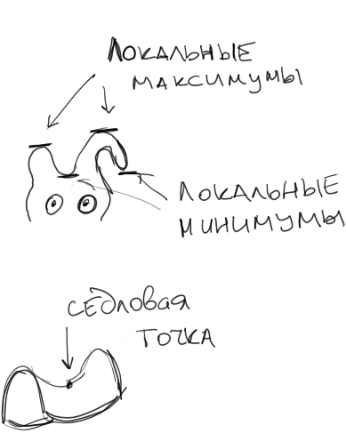
Extremum of the function
Let the function f be given:U⊂ Rn → R for x∈ U. The point x0 is the local maximum of the function if f(x0)≤f(x) in some neighborhood around the point x0. The point x0 is the local minimum of the function if f(x0)≥f(x) in some neighborhood around the point x0.
Let be given a function f: U ⊂ Rn → R differentiable at the point x0 and the point x0 is a local extremum, then x0 is a critical point, i.e. ∇f(x0)=0, so all partial derivatives of the first order at this point are zero.
If all partial derivatives are zero, then the point x0 is not necessarily a critical point, but can be a saddle point.
Hessian of the function
Let's give a function f: U ⊂ Rn → R belonging to the second class. The Hesse Matrix f at the point x0 is a symmetric matrix:
d2f/dx1dx1(x0) ... d2f/dx1dxn(x0) Hf(a) = ... ... ... d2f/dxndx1(x0) ... d2f/dxndxn(x0)
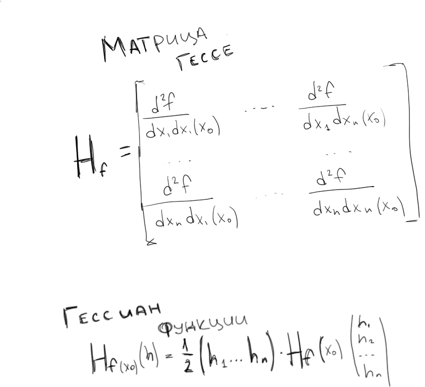
The Hessian of the function f at point x0 is the following function:
Hf(x0)(h) = ½(h1 ... hn)⋅Hf⋅(x0)⋅(h1 ... hn)T
Let's give the function f : U⊂ Rn → R, f∈ C3 and U is an open interval. Consider the critical point x0 ∈ U (∇f(x0)=0):
x0 is the point of the local minimum if Hf(x0)(h) > 0 for any h≠ 0.
x0 is a point of the local maximum if Hf(x0)(h) < 0 for any h≠ 0.
x0 is a saddle point if Hf(x0)(h) ≠ 0 for any h≠ 0.
Lagrange multipliers
This method was introduced to solve the problem of finding extremum points on a closed set D. The methods described above are suitable for finding the extremum on an open set, so the problem is divided into two: the first is to find the extremes in the open interval, the second is to find the extremes on the boundary of the interval, comparing the obtained extremes, we will find the extremes of the function on the set D.
Let's introduce the concept of a level surface, a level surface of a function f is a set of points in space where the function is equal to a given value, you could see this earlier, for example, in maps where the isolines the height above sea level is indicated, each such contour is the surface of the level. Level H surface this is the set of points f(xi, ...) = h
Let's give two functions of the first class f : U⊂ Rn → R and g : U ⊂ Rn → R. The point a ∈ U and g(a) = c and the surface of the level "c" of the function g are denoted by S. If the function fs at point a is the maximum or minimum, then ∇g(a) will be perpendicular to S at point a, which means that there is a certain number such that f(a)=g(a).
Example
It is necessary to find the maximum and minimum of the function f(x,y,z) = x + 2y + 3z on the section formed by the intersection of the cylinder x2 + y2 = 2 and the plane y + z = 1
In this example, we have a limitation of two functions, so there will be 2 multipliers, in general, we are interested in the result:
∇f(x,y,z)=λ∇g(x,y,z)+μ∇h(x,y,z)
where g(x,y,z) = x2 + y2 - 2 and h(x,y,z) = y+ z - 1
more details:
df/dx = λ⋅dg/dx + μ⋅dh/dx
df/dx = λ⋅dg/dy + μ⋅dh/dy
df/dx = λ⋅dg/dz + μ⋅dh/dz
having solved this system of equations, we get two critical points: P(1,-1,2) and Q(-1,1,0) to check, which of them is the maximum and which is the minimum, it is necessary to calculate the value of the function:
f(1,-1,2) = 5
f(-1,1,0) = 1
Therefore, the maximum is at point P, the minimum is at point Q.