Mathematical description
Looking at the law of distribution, we can understand what is the probability of an event, we can say what is the probability that a group of events will occur, and in this article we will look at how to translate our conclusions "by eye" into a mathematically sound statement.
An extremely important definition: mathematical expectation is the area under the distribution graph. If we are talking about a discrete distribution - this is the sum of events multiplied by the corresponding probabilities, also known as moment:
(2) E(X)=Σ(pi•Xi) E - from the English word Expected (waiting)
For mathematical expectation, the equalities are valid:
(3) E(X + Y) = E(X) + E(Y)
(4) E(X•Y) = E(X) • E(Y)
Moment of degree k:
(5) νk = E(Xk)
The central moment of degree k:
(6) μk = E[X - E(X)]k
Average value
Average value (μ) the distribution law is the mathematical expectation of a random variable (a random variable is an event), for example, how many average visitors come to the store per hour:
| Number of visitors | 0 | 1 | 2 | 3 | 4 | 5 | 6 |
| Number of observations | 58 | 79 | 0 | 59 | 84 | 8 | 112 |
| Table 1. Number of visitors per hour | |||||||
To find the average value of all the results, you need to add everything together and divide by the number of results:
μ = (58 • 0 + 79 • 1 + 0 • 2 + 59 • 3 + 84 • 4 + 8 • 5 + 112 • 6) / 400 = 1304/400 = 3.26
We can do the same using formula 2:
μ = M(X) = Σ(Xi•pi) = 0 • 0.15 + 1 • 0.2 + 2 • 0 + 3 • 0.15 + 4 • 0.21 + 5 • 0.02 + 6 • 0.28 = 3.26 Moment of the first degree, formula (5)
Actually, formula 2 is the arithmetic mean of all values
Total: on average, 3.26 visitor per hour
| Number of visitors | 0 | 1 | 2 | 3 | 4 | 5 | 6 |
| Probability (%) | 14.5 | 19.8 | 0 | 14.8 | 21 | 2 | 28 |
| Table 2. The law of distribution of the number of visitors | |||||||
Deviation from the mean
Look at this distribution, we can assume that on average the random variable is 100±5, because it seems that there are incomparably more such values than those that are less than 95 or more than 105:
The average value according to the formula (2): μ = 99.95, but how to calculate how far all values are from the average? You should be the entry 100±5 is familiar. To get this value ±, we need to define a range of values around the mean. And we could use the "difference" between the mean and random variables as a distance measure:
(7) xi - μ
but the sum of such distances, and therefore any derivative of this number, will be zero, so the square of the differences was chosen as the measure between the values and the average value:
(8) (xi - μ)2
Accordingly, the average distance value is the mathematical expectation of the squares of the distance:
(9) σ2 = E[(X - E(X))2] Since the probabilities of any distance are equal, the probability of each of them is 1/n, from where: (10) σ2 = E[(X - E(X))2] = ∑[(Xi - μ)2]/n It is also the formula of the central moment (6) of the second degree
σ is squared, because instead of distances we took the square of distances. σ2 is called variance. The root of the variance it is called the mean square deviation, or the standard deviation, and it is used as a measure of the spread:
(11) μ±σ
(12) σ = √(σ2) = √[∑[(Xi - μ)2]/n]
Returning to the example, let's calculate the standard deviation for graph 2:
σ = √(∑(x-μ)2/n) = √{[(90 - 99.95)2 + (91 - 99.95)2 + (92 - 99.95)2 + (93 - 99.95)2 + (94 - 99.95)2 + (95 - 99.95)2 + (96 - 99.95)2 + (97 - 99.95)2 + (98 - 99.95)2 + (99 - 99.95)2 + (100 - 99.95)2 + (101 - 99.95)2 + (102 - 99.95)2 + (103 - 99.95)2 + (104 - 99.95)2 + (105 - 99.95)2 + (106 - 99.95)2 + (107 - 99.95)2 + (108 - 99.95)2 + (109 - 99.95)2 + (110 - 99.95)2]/21} = 6.06
So, for graph 2 we got:
X = 99.95±6.06 ≈ 100±6, which is slightly different from the received "by eye"
Quantile
Graph 4. Distribution function. 4-quantile or quartile
Graph 5. Distribution function. 0.34-quantile
To analyze the distribution function, the concept of quantile was introduced. A quantile is a random variable at a given probability level, i.e.: a quantile for a probability level of 50% is a random variable on a probability density graph that has a probability of 50%. In the example with graph 3, the quantile of the level 0.5 = 99 (the nearest value, since the distribution is discrete and events with a value of 99.3 simply do not exist)
- 2-quantile median
- 4-quantile - quartile
- 10-quantile - decile
- 100-quantile - percentile
That is, if we are talking about a decile (10-quantile), it means that we have divided the graph into 10 parts, which corresponds to nine lines, and for each decile we have found the value of a random variable.
Also, the notation x-quantile is used, where x is a fractional number, for example, 0.34-quantile, such an entry means the value of a random variable when p = 0.34.
For a discrete distribution, the quantile must be chosen as follows: the quantile guarantees the probability, therefore, if the calculated the quantile does not match one and the values, it is necessary to choose a smaller value.
For example, we have a discrete distribution of 1325 values, given that each value has a probability of 1/1325, the 10th quantile will have a value that does not exceed 10% of 1325, that is, a value equal to or less than 132.5.
Building intervals
Quantiles are used to construct confidence intervals, which are necessary for the study of statistics of more than one specific event (for example, interest is a random number = 98), and for a group of events (for example, interest is a random number between 96 and 99). The confidence interval is of two types: one-sided and two-sided. The parameter of the confidence interval is the confidence level. The confidence level means the percentage of events that can be considered successful.
Two-way confidence interval
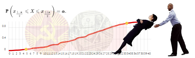
The two-way confidence interval is constructed as follows: we set the significance level, for example, 10%, and select an area on the graph so that 90% of all events will fall into this area. Since the interval is two-sided, we cut off 5% on each side, i.e. we are looking for the 5th percentile, the 95th percentile and the values of the random variable between them will be the confidence area, values outside the confidence area are called "critical area"
Confidence interval
The left-sided and right-sided confidence intervals are constructed similarly to the two-sided one: for the left-sided interval, we find the percentile of the level ['one' minus 'significance level']. Thus, to construct a confidence left-sided interval of the significance level of 4%, we need to find the fourth percentile and everything on the right is a confidence interval, everything on the left is a critical area.
Total
The average value is the mathematical expectation of a random variable, found by the formula:
μ = E(X) = Σ(pi•Xi)
The standard deviation is the mathematical expectation of the distance of values from the average, is found by the formula:
σ = √(σ2) = √[∑[(Xi - μ)2]/n]
n-quantile - division of the distribution function into n equal segments, the main types of quantiles:
- 2-quantile - median
- 4-quantile -quartiles
- 10-quantile - deciles
- 100-quantile - percentiles
The confidence interval of the α level is a section of the probability function containing α of all possible values. The two-way confidence interval is constructed by clipping (1-α)/2 on the right and left. The left- sided and right-sided confidence intervals are constructed by clipping areas (1-α) left and right respectively.
Construct a distribution series
Suppose we have 100 values and all are different, for example: the body weight of Somali pirates. It is inconvenient to process such a set of data, we cannot even present them on a regular graph. Therefore, we need to categorize the available data and for this we do the following:
Let's write down our data in the table:
| 105 | 118 | 56 | 110 | 102 | 95 | 99 | 118 | 97 | 51 |
| 81 | 105 | 89 | 103 | 68 | 103 | 109 | 89 | 53 | 62 |
| 115 | 58 | 63 | 58 | 67 | 74 | 107 | 71 | 55 | 86 |
| 78 | 82 | 64 | 79 | 75 | 77 | 106 | 72 | 88 | 67 |
| 76 | 99 | 85 | 82 | 77 | 92 | 94 | 118 | 97 | 115 |
| 52 | 64 | 68 | 102 | 65 | 54 | 72 | 65 | 63 | 51 |
| 109 | 110 | 83 | 95 | 105 | 116 | 56 | 54 | 118 | 111 |
| 103 | 60 | 54 | 79 | 77 | 51 | 58 | 100 | 61 | 73 |
| 63 | 74 | 62 | 71 | 61 | 63 | 89 | 85 | 55 | 115 |
| 65 | 69 | 101 | 89 | 103 | 59 | 116 | 69 | 77 | 58 |
| Table 3. Weight of Somali pirates | |||||||||
We will divide the data into groups, to begin with, I suggest splitting it into six intervals:
Find out the maximum and minimum values, subtract them from each other and divide by the number intervals - received segments:
Maximum value: 118
Minimum value: 51
Difference: 118 - 51 = 67
Interval length: 67 / 6 = 11.17
Now let's count the number of pirates (weights, I mean) in each interval:
| # | Interval | Number of elements |
|---|---|---|
| 1. | 51 - 62.17 | 22 |
| 2. | 62.17 - 73.34 | 20 |
| 3. | 73.34 - 84.51 | 15 |
| 4. | 84.51 - 95.68 | 12 |
| 5. | 95.68 - 106.85 | 16 |
| 6. | 106.85 - 118.02 | 15 |
| Table 4. Number of elements in intervals | ||
Voila, our distribution on the graph:
Bonus
It is better to take the intervals as integers, so if with the selected number of intervals the size comes out as a non-integer, then you can expand the range of values, for example:
The interval value is 11.17, the number is not an integer, so pushing back the upper bound:
The remainder of the division: [(118 - 51) / 6] = 1
Move to: 5
New range: [51;123]
The range can be moved both up and down, but preferably in both directions.
Tip
It is customary to divide the distribution into 7-8 intervals, but in each specific situation You can choose a great number of intervals, however, as well as make them of different lengths.
List of parameters
So, here is a list of the main parameters of the discrete distribution law:
| Name | Symbol | Formula |
|---|---|---|
| Mathematical expectation (average) | E(X) | Σ(pi•Xi) |
| Central moment (standard deviation) | σx | σ = √(σ2) = √[∑[(Xi - μ)2]/n] |
| Interval length | R | max(x) - min(x) |
| Fashion | mo | max P(x = mo) |
| 1st quantile | - | F(x) = 0.25 |
| Median | me | F(x) = 0.5 |
| Decile | - | F(x) = 0.1 |
| Table 5. Basic parameters of the discrete distribution law | ||
Histogram template in OpenOffice Calc
File histogram_mock.ods contains a histogram construction template.